| 1. 80-metre offset paraboloid (June 2006) 2. 90-metre offset paraboloid (May 2009) 3. RT32 with OCRAp/f (pointing and gain) (June 2005) 4. Follow-up of the above (OCRA-f) (July 2006) 5. Properties of the RT32 enlarged to 36 m (in Polish; January 2009) 6. A 90 m Transit Radio Telescope: Offset or Symmetrical? (September 2009) 7. A 100 m Radio Telescope: Some Optical Properties (January 2010) 8. Optical Coma Structure Demonstrated with OptiCass (June 2011) |
Here is yet another.
|
A month ago or so (in April 2011) Maciej Mikołajewski of the Department of Astronomy and Astrophysics hit on the novel idea of choosing an aplanatic design for the new telescope. The design, known as Ritchey-Chretien (RC), is quite popular among large optical telescopes but apparently never has been used in radio astronomical practice. This report focuses on comparison of properties of a radio telescope of RC type with the classical Cassegrain. The main feature of the RC telescope is that its both mirrors are hiperboloidal. Coefficients of the conics are chosen so that both the spherical aberration and coma, to third order, are said to be absent in such a telescope. The present study, like those earlier ones, is based on ray tracing simulations performed with the OptiCass program. Ray tracing in this program, however, is carried out specifically according to a classical Cassegrain geometry, where the primary mirror is paraboloidal and secondary is hyperboloidal, therefore it required considerable modifications. In the following the needed modifications are described and some computations presented. They lead to the conclusion that RC telescope performes better than CC telescope in number of properties (like smaller losses for offset feeds, smaller distortions, sidelobes etc.). Even though the improvements are not great, in view that the construction of an RC radio telescope (unlike optical telescope) would not pose any extra difficulties compared to similar CC telescope, the RC design should be seriously considered for the RTH telescope. Also, it seems that certain modifications of the RC idea would ensure still better performance in certain aspects. |
Table of contents
|
K1 = –1 –
2(1 + β)/[m2(m – β)] K2 = –[(m + 1)/(m – 1)]2 – 2 m(m + 1)/[(m – β)(m – 1)3], |
(1) |
| m = (1 + β)D/d – 1, | (2) |
|
K1 = –1 –
2(1 – η)/m3 K2 = –[(m + 1)/(m – 1)]2 – 2mf/[(f – f1)(m – 1)3] = –1 – 2[m(2m – 1) + 1 – η]/(m – 1)3, | (3) |
Having calculated these coefficients, mirror surfaces can then be described by equations of the form:
| x2 + y2 = 2Rz – (1 + K)z2, | (4) |
| R2 = 2f1/(m – 1), | (5) |
| R2 = 2(f – f1 – h)/[(mf + h)/(f – f1) – 2]. | (6) |
The vertex radii of curvature, R1 and R2, are the same for classical Cassegain and corresponding RC, but the conic constatnts are different and for classical Cassegrain they are:
|
K1 = –1 K2 = –[(m + 1)/(m – 1)]2. |
(7) |
The following table, Table 1., and Fig. 1. present example sets of coefficients of classical and two RC designs in which the secondary diameters are very nearly equal. The first two (i.e. Classical and Solution A) are used in this report for performance comparison basing on simulations with the technique of ray-tracing. The Solution A was obtained with certain modifications of Eqs. (1) and (2) and Solution B strictly according to these equations but starting with d = 8.94472 m to get final RC secondary diameter of 9.0 m. The Solution B gives considerably sharper focus, but in our case both solutions (A and B) seem equally suitable, and in certain respects Solution A is better than Solution B. This itself suggests that there must be a considerable room for choice of the conic constants and good chances for finding other solutions of interest that are far removed from original Ritchey and Chretien ideas. We shall return to this important aspect later in this report.
Table 1: Classical Cassegrain and
Ritchey-Chretien Radio Telescope Data
 Aperture diameter, D                                     90.000 m
 Focal length of primary mirror, f                        31.500 m
 Focal ratio of primary mirror, f/D                        0.350
 Subreflector diameter, d                                  9.000 m
 Height of secondary focus above main dish vertex, h       1.000 m

                                            Classical      Ritchey-Chretien
                                                        Solution A  Solution B
 Subreflector radius                         4.50000      4.49950    4.50000 m
 Secondary magnification, m                  9.24790      9.31154    9.30740
 Prime focus to subreflector vertex, f1       2.97622      2.95785    2.95904 m
 Secondary focus to hyperboloid vertex, f2   27.52378     27.54215   27.54096 m
 Secondary interfocal length                30.50000     30.50000   30.50000 m
 R1                                         63.00000     63.00000   63.00000 m
 K1                                         -1           -1.00255   -1.002394
 R2                                          6.67412      6.62745    6.63046 m
 K2                                         -1.54377     -1.57496   -1.575293
|
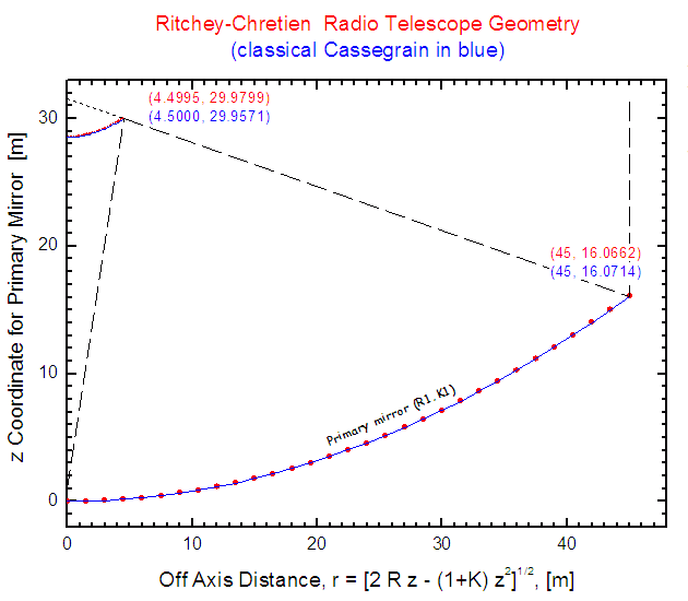
| Fig. 1: Example of geometry and dimensions of Ritchey-Chretien (in red; Solution A) and classical Cassegrain (in blue) telescopes for RTH. This figure is to scale. Note the smallness of differences in mirror shapes: the depth of both RC mirrors is smaller than CC ones by about 5 mm only (subreflector depths are 1.4334 m and 1.4380 m, for RC and CC, respectively). |
The program OptiCass, developed
a few years ago has a procedure
for tracing ray paths between a feed and aperture plane with reflections
from a hiperboloidal subreflector and paraboloidal main mirror.
The procedure returns initial and final direction cosines, the pathlength
and coordinates of the reflection point on paraboloid and coordinates
on the aperture plane. These coordinates on aperture are used to transform
(DFT) amplitude distribution into the telescope power pattern.
Almost all algorithms of this scheme had to be worked out anew because
of different shape of main mirror and the fact that in RC the rays parallel
to main mirror axis are no more reflected towards the primary focus.
Still the general scheme, as described
there, remains valid for the new
procedure (provided the word 'paraboloid' there is replaced with 'primary
hyperboloid'). The weakness of this modified procedure is that
the solutions for rays very close to the vertices tend to be unstable
when the conic coefficient K1 nears –1 (i.e. the main dish turnes
into paraboloid). Therefore, this version of OptiCass cannot be considered
a true generalization of its progenitor, and
hence it was named OptiCassRC. Nevertheless, OptiCassRC can be used
to simulate also a classical Cassegrains by setting main mirror
conic constant very, very close to –1 (with e.g. K1 = –1.000001
90-m quasi-paraboloid depth of our RTH is smaller than true paraboloid
depth by only 2 μm or 2E–6 m). This quasi-paraboloidal
mode was used as a final check of the correctness of the ray tracing
algorithm implementation in the new version of OptiCass.
Ray Tracing in an RC Telescope
| Fig. 2: The height of feed above the secodary focal plane (towards the subreflector) for which the least aberration (shown in Fig. 4) and spillover losses are found while simultaneously adjusting the direction of feed power pattern (Fig. 3). |
| Fig. 3: Correction of the direction of feed (with respect to direction to the centre or vertex of subreflector) for which the least aberration and spillover losses (shown in Fig. 4) are found. |
| Fig. 4: Losses of antenna gain as a function of feed lateral offset optimized in placement in z-coordinate and direction as shown in Fig. 2 and Fig. 3. |
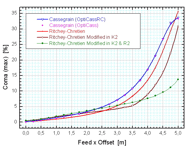
| Fig. 5: Height of first sidelobe and comatic distortion as a function of lateral offset at optimal placement and orientation of feed (see Fig. 2 and Fig. 3). |
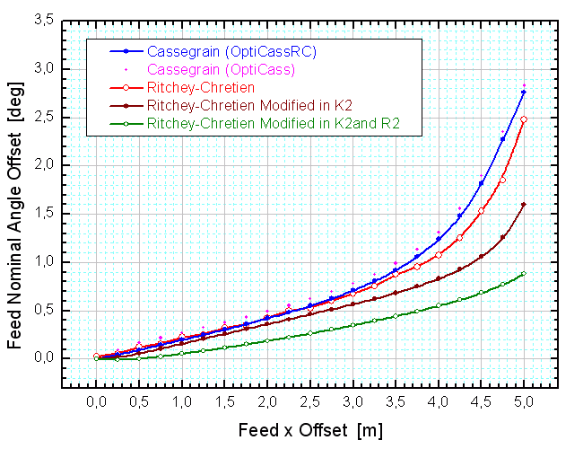
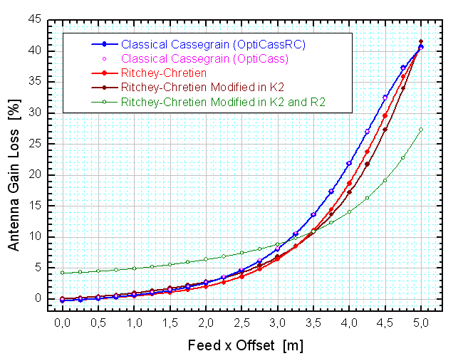
The results presented in Figs. 4 and 5 seem to prove that the RC design performes
indeed significantly better than Cassegrain in respect of aberration losses
as well as of magnitudes of coma and first sidelobe.
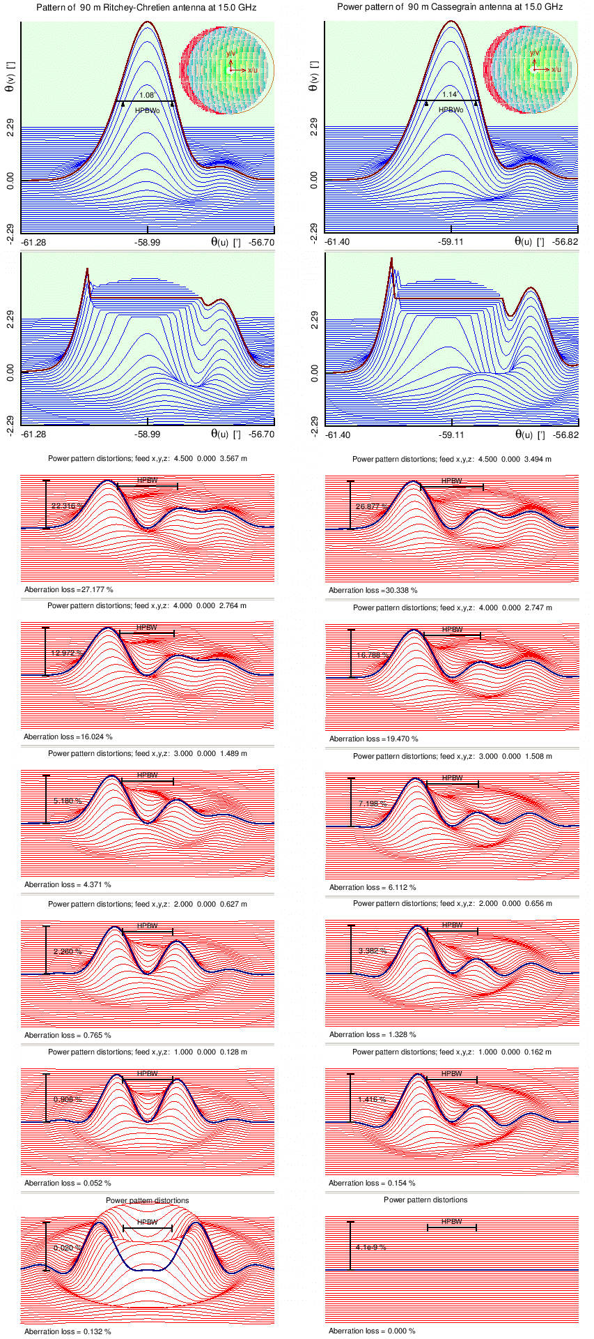
RC Solution A Classical Cassegrain | RC Solution B |
|

|
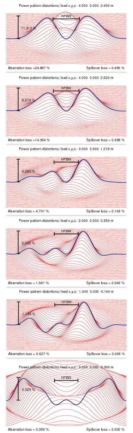
| Fig. 6: (Left figure, RC Solution A and Classical Cassegrain) Distortions of power pattern of Ritchey-Chretien (left panels) and classical Cassegrain (middle panels). The distortions (shown in red) represent difference between power pattern at given offsets and offset-free power pattern. Note the different scales of each panel as indicated next to the vertical bars (readable here). The two uppermost panels (in blue) contain the patterns themeselves at largest analysed feed offset (4.5 m), the lower one showing more details of bottom part of the same pattern (main beam being here cut-off at 9% of the maximum power). Click on this image to see it in a higher resolution. The three figures on the right, RC Solution B, contain similar results for RC but using Solution B of Table 1. Here only distortions at feed offsets of 4.5 and 0 m are shown. Note that at 0 m offset (all bottom panels) this solution has an order of magnitude smaller residuals than the Solution A, but for nonzero offsets their patterns are very much the same. The circular inset at top right of the three upper panels represents all the rays traced, with their phases (colour) and amplitudes (brightness), as seen on aperture plane after traversing the path from feed (rays reflected from the secondary but missing the primary mirror contribute to spillover loss and are marked red). |
Table 2A: Ritchey-Chretien and
Classical Cassegrain Tolerances
|
Feed placed at focus
|
* These values include (the largest) contribution
to gain loss due to
decentered illumination
of the aperture by an angularly offset feed.
Table 2B: Ritchey-Chretien and
Classical Cassegrain Tolerances
|
Feed placed off axis at x = 4 m Ritchey-Chretien (RC): z_feed = 2.764 m, feed x-z_tilt = 1.067° RC Class. Subreflector z_offset -0.002 m 0.41 -1.36 Subreflector z_offset +0.002 m 1.64 1.44 Subreflector x_offset -0.005 m -2.27 -3.21 Subreflector x_offset +0.005 m 2.96 3.76 Subreflector y offset ±0.005 m 0.48 0.45 Subreflector x-z_tilt -0.02° 1.24 1.40 Subreflector x-z_tilt +0.02° -1.18 -1.38 Subreflector y-z_tilt ±0.2° -0.01 0.64 Feed z_offset -0.1 m 0.66 0.72 Feed z_offset +0.1 m 0.69 0.62 Feed x-z_tilt offset -1° 1.57* 2.27* Feed x-z_tilt offset +1° 1.50* 2.22* Feed y-z_tilt ±1° 1.34* 2.20* |
* These values include (the largest) contribution to gain
loss due to
decentered illumination of the aperture by an angularly
offset feed.
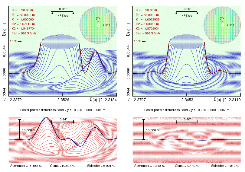
From the previous sections it can be concluded that RC idea does not give as significant improvements as could be hoped from experience at optical wavelengths. The reader might take this as an indicatation of a flaw in our implementation of the RC idea itself. However, our algorithm, as implemented in OptiCassRC, produces very nice improvement over classical Cassegrain at very high frequencies, say 100 GHz or higher. Here, in Fig. 7a., is an example of performance of the two designs at λ = 0.3 mm (1000 GHz).
| Fig. 7a: Left: Off axis power pattern of classical Cassegrain telescope and, Right:, the same for Richey-Chretien at (unrealistically short) wavelength of 0.3 mm. Both the aberration losses and distortions are smaller in RC telescope by an order of magnitude. |
Further ray tracing simulations at range of frequencies exhibited quite
interesting behaviour of RC design which seems to be really superior
to classical solutions. Over a wide span of frequencies it does have
smaller aberration losses (those due to phase errors), distortions
and sidelobes than Cassegrain.
| Fig. 7b: Off axis characteristics of the 90-metre radio telescope computed for classical Cassegrain (CC) and Richey-Chretien (RC) designs as functions of observing frequency. Note the excellent performance of RC above 100 GHz. |
Here are more systematic results obtained for three telescopes, the other
two having the same optical geometries as RTH90 but scaled up and down
by the factor of 10.
| Fig. 7c |
| Fig. 7d |
| Fig. 7e |
Thus, it seems, as we go towards longer wavelengths the RC system gradually
loses its effectiveness.
| K2 = (K1 + 1)(D/d)4[R2/(2f)]3 – [(m + 1)/(m – 1)]2. | (8) |
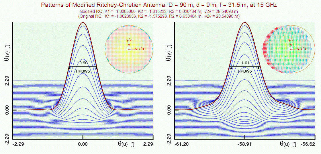
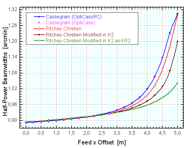
Fig. 8. and Fig. 9. give more details on performance of so modified RC telescope. Compare also the HPBW of 1.01 arcminutes here with 1.09 to 1.14 arcminutes of RC and classical Cassegrain in Fig. 6.
| Fig. 8: Left: Power pattern of modified Richey-Chretien telescope at best position near focus (31 cm below it), Right: The same for the feed placed 4.5 m off axis. (The quantity 'v2v' is the vertex to vertex distance between the two mirrors.) |
| Fig. 9: Off axis pattern distortions in modified RC of Fig. 8. |
Results presented in this report so far, for speed of computing, were
obtained with a small number of rays traced (about 1300) and with low
resolution (80 pixels in u/x direction) of final patterns. Here are similar
results computed with these parameters being nearly maximum possible
in OptiCass presently (over 11000 rays and 200 pixels). In addition,
both versions of the program, OptiCass and OptiCassRC, were somewhat improved
with respect to initial ray distribution on the aperture. Earlier the rays
covered the area up to half their spacing away from dish edge; now they
go up to half the spacing beyond the edge (the rays close to the edge
are waighted, besides the usual illumination function, by the approximate
fraction of circular area around them that remains on the dish). Therefore,
these data should be considered more realistic.
The new results are given in the form of Figs. 10. to 15. They all were computed for wavelngth of 2 cm. Each of the four curves correspond to a set of conic parameters detailed in Table 3.
Table 3: Conic Constants of Four
Variants of Mirror Curvature of 90-metre RTH
                                K1          K2     R2 [m]  v2v [m]
Classical Cassegrain      -1.00000001 -1.5437704 6.67412 28.52378
Ritchey-Chretien          -1.0023936  -1.5752934 6.63046 28.54096
Modified Ritchey-Chretien -1.0065000  -1.6152331 6.63046 28.54096
Modified Ritchey-Chretien -1.0065000  -1.6118407 6.53000 28.54096
|
| Fig. 10: The height of feed above the secodary (final) focal plane (towards the subreflector) for which the least aberration and spillover losses (shown in Fig. 12) are found while simultaneously adjusting the direction of feed power pattern (Fig. 11). |
| Fig. 11: Correction of the direction of feed (with respect to direction to the centre or vertex of subreflector) for which the least aberration and spillover losses (shown in Fig. 12) are found. |
| Fig. 12: Losses of antenna gain as a function of lateral feed offset optimized for z-coordinate and direction as shown in Fig. 10 and Fig. 11. |
| Fig. 13: Height of comatic distortion as a function of lateral offset at optimal placement and orientation of feed (see Fig. 10 and Fig. 11). |
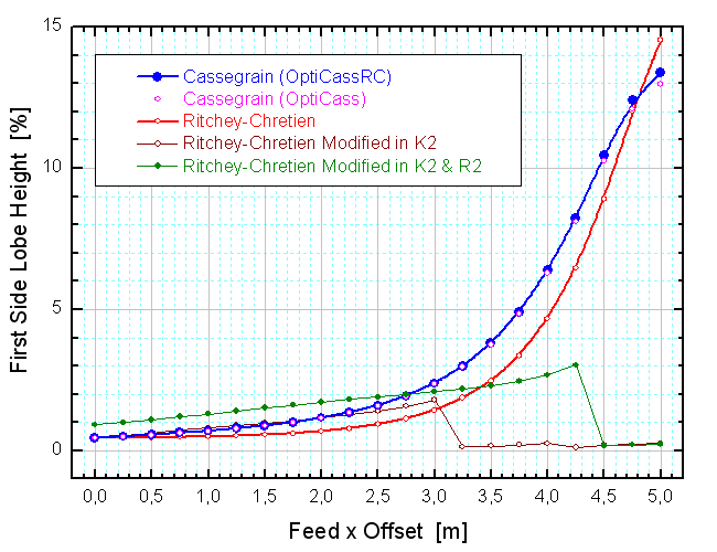
| Fig. 14: Height of first sidelobe as a function of lateral offset at optimal placement and orientation of feed (see Fig. 10 and Fig. 11). The sidelobe is measured along the direction of feed offset on both sides of the main lobe and the higher value is taken. In the case of the two modified RCs the sidelobe on the side further off telescope symmetry axis, as it grows with incerasing offset, it gradually merges in the telescope main beam to disappear altogether, so that there is a downward jump and the values shown at greater offsets represent level of the second sidelobe. |
| Fig. 15: Half-power beamwidth as a function of lateral offset at optimal placement and orientation of feed (see Fig. 10 and Fig. 11). |
| K1 + 1 = 4 (m2 + β) (1 + β)/[m (m – β)]2 | (9) |
Ray tracing simulations indicate that the gain losses for such a design and for feed offsets smaller than about 3 m are slightly smaller than with heretofore analysed solutions, and similar or somewhat worse above this offset (although still better than in the case of CC). However, see note in the last paragraph about insufficiency of these simulations.
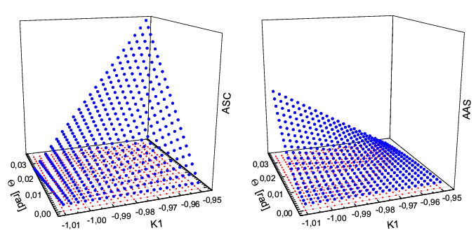
According to theory the extent of angular coma (ASC or sagittal coma, to be precise) and angular astigmatism (AAS) in a two mirror telescope whose mirrors fulfill the condition of absence of spherical aberration, are as follows (see Tab. 6.7 of Schroeder):
| ASC = [1 + (K1 + 1)m2(m – β)/(2(1 + β))]Θ/(4 m f/D)2 | (10) |
| AAS = [(m2 + β)/(m(1 + β)) – (K1 + 1)m(m – β)2/(4(1 + β)2)]Θ2/(2 m f/D) | (11) |
These functions for RTH geometry are plotted in Fig. 16. for a range of the angle and the K1 constant.
| Fig. 16: Coma (left) and astigmatism (right) as a function of the angular offset (the Θ range is 0 to 2 deg and it corresponds to about 0 to 5 m of feed lateral offset) and of the primary conic constant, K1, for 90-metre radio telescope. Coma zeroes a little below K1 = –1.002 and astigmatism zeroes at about K1 = –0.95. Note that where astigmatism is zero coma is about twice as big as astigmatism is at coma's zero. |
Since, as evidenced by this figure, theoretical coma increases faster
towards K1 for
which astigmatism gets to zero than astigmatism decreases, one should
not expect improvement of RTH telescope properties of anastigmat aplanat
type. However, the above mentioned ray tracing simulations suggest that
there is certain improvement. Unfortunately, these simulations cannot
be taken as conclusive since geometry of such aplanat is too different
from classical Cassegrain (the main mirror is not completely illumined
by subreflector). Although we believe the results from simulations are not
far from truth, this type of design would need further study to be
seriously considered as a candidate for RTH.
Posted in May, 2011, by KMB
Last updated: July 27, 2011
-t.gif)
-t.gif)
-t.gif)
-t.gif)
.gif)
.gif)
.gif)
.gif)