Preprint of a paper published in Classical and Quantum Gravity,
vol. 20, No 17 (7 September 2003), S665–S676

All-sky upper limit for gravitational
radiation from spinning neutron stars

P Astone, D Babusci, M Bassan§, K M Borkowski#, E Coccia§, S D'Antonio§, V Fafone, G Giordano, P Jaranowski£, A Królak$ * &, A Marini, Y Minenkov§, I Modena§, G Modestino, A Moleti§, G V Pallottino||, M Pietka£, G Pizzella, L Quintieri, A Rocchi§, F Ronga, R Terenzi+ and M Visco+

 Istituto Nazionale di Fisica Nucleare INFN, Rome, Italy
 Istituto Nazionale di Fisica Nucleare INFN, Frascati, Italy
§ University of Rome "Tor Vergata" and INFN, Rome II, Italy
|| University of Rome "La Sapienza" and INFN, Rome, Italy
¶ University of Rome "Tor Vergata" and INFN, Frascati, Italy
+ IFSI-CNR and INFN, Rome
# Centre for Astronomy, Nicolaus Copernicus University, Torun, Poland
£ Institute of Theoretical Physics, University of Bialystok, Bialystok, Poland
$ Jet Propulsion Laboratory, Pasadena, USA

Abstract

We present results of the all-sky search for gravitational-wave signals from spinning neutron stars in the data of the EXPLORER resonant bar detector. Our data analysis technique was based on the maximum likelihood detection method. We briefly describe the theoretical methods that we used in our search. The main result of our analysis is an upper limit of 2×10-23 for the dimensionless amplitude of the continuous gravitational-wave signals coming from any direction in the sky and in the narrow frequency band from 921.00 Hz to 921.76 Hz.


1  Introduction

A unique property of the gravitational-wave detectors is that with a single observation resulting in one time series one can search for signals coming from all sky directions. In the case of other instruments like optical and radio telescopes, to cover the whole or even part of the sky requires a large amount of expensive telescope time as each sky position needs to be observed independently. The difficulty in the search for gravitational-wave signals is that they are very weak and they are deeply buried in the noise of the detector. Consequently the detection of these signals and interpretation of data analysis results is a delicate task. In this paper we present results of an all-sky search for continuous sources of gravitational radiation. A prime example of such a source is a spinning neutron star. A signal form such a source has definite characteristics that make it suitable for application of the optimal detection techniques based on matched filtering. Moreover such signals are stable as a result of the stability of the rotation of the neutron star and they will be present in the data for time periods much longer than the observational interval. This enables a reliable verification of the potential candidates by repeating the observations both by the same detector and by different detectors. To perform our all-sky search we have used the data of the EXPLORER [1] resonant bar detector. The directed search of the galactic center with the EXPLORER detector has already been carried out and an upper limit for the amplitude of the gravitational waves has been established [2].
Our paper is divided into two parts. In the first part we summarize the theoretical tools that we use in our analysis and in the second part we present results of our all-sky search. The main result of our analysis is an upper limit of 2×10-23 for dimensionless amplitude of gravitational waves originating from continuous sources located in any position in the sky and in the frequency band from 921.00 Hz to 921.76 Hz.
The data analysis was performed by a team consisting of Pia Astone, Kaz Borkowski, Piotr Jaranowski, Andrzej Królak and Maciej Pietka and was carried out on the basis of Memorandum of Understanding between the ROG collaboration and Institute of Mathematics of Polish Academy of Sciences. More details about the search can be found on the website: www.astro.uni.torun.pl/~kb/AllSky/AllSky.html.

2  Data analysis methods

In this section we give a summary of data analysis techniques that we used in the search. The full exposition of our method is given in Ref. [6].

2.1  Response of a bar detector to a continuous gravitational-wave signal

Dimensionless noise-free response function h of a resonant bar gravitational-wave detector to a weak plane gravitational wave in the long wavelength approximation [i.e., when the size of the detector is much smaller than the reduced wavelength l/(2p) of the wave] can be written as a linear combination of the wave polarization functions h+ and h×:
h(t) = F+(t) h+(t) +F×(t) h×(t),
(1)
where F+ and F× are called the beam-pattern functions and can be written as
F+(t)
=
a(t)cos2y+b(t)sin2y,
F×(t)
=
b(t)cos2y-a(t)sin2y,
(2)
where y is the polarization angle of the wave and
a(t)
=
1

2
(cos2g-sin2gsin2f) (1+sin2d)cos[2(a-fr-Wr t)]
+ 1

2
sin2gsinf(1+sin2d)sin[2(a-fr-Wr t)]
- 1

2
sin2gsin2fsin2dcos(a-fr-Wr t)
+ 1

2
sin2gcosfsin2dsin(a-fr-Wr t)
+ 1

2
(1-3 sin2gcos2f) cos2d,
b(t)
=
-sin2gsinfsindcos[2(a-fr-Wr t)]
+ (cos2g-sin2gsin2f) sindsin[2(a-fr-Wr t)]
- sin2gcosfcosdcos(a-fr-Wr t)
- sin2gsin2fcosdsin(a-fr-Wr t).
(3)
In Eqs. (2) and (3) the angles a and d are respectively right ascension and declination of the gravitational-wave source. The geodetic latitude of the detector's site is denoted by f, the angle g determines the orientation of the bar detector with respect to local geographical directions: g is measured counter-clockwise from East to the bar's axis of symmetry. The rotational angular velocity of the Earth is denoted by Wr, and fr is a deterministic phase which defines the position of the Earth in its diurnal motion at t=0 (the sum fr+Wrt essentially coincides with the local sidereal time of the detector's site, i.e., with the angle between the local meridian and the vernal point).
We are interested in a continuous gravitational wave, which is described by the wave polarization functions of the form
h+(t) = h0+ cosY(t),     h×(t) = h sinY(t),
(4)
where h0+ and h are independent constant amplitudes of the two wave polarizations. These amplitudes depend on the physical mechanisms generating the gravitational wave. In the case of a wave originating from a spinning neutron star these amplitudes can be estimated by ([3])
ho £ 4.23×10⁻²³ æ
è
e

10-5
ö
ø
æ
è
I

1045 g cm2
ö
ø
æ
è
1 kpc

r
ö
ø
æ
è
f

1 kHz
ö
ø
2

 
,
(5)
where I is the neutron star moment of inertia with respect to the rotation axis, e is the poloidal ellipticity of the star, and r is the distance to the star. The value of 10-5 of the parameter e in the above estimate should be treated as an upper bound. In reality it may be several orders of magnitude less.
The phase Y of the wave is given by
Y(t)
=
F0 + F(t),
F(t)
=
s1
å
k=0 
wk tk+1

(k+1)!
+ n0·rSSB(t)

c
s2
å
k=0 
wk tk

k!
.
(6)
In Eq. (6) the parameter F0 is the initial phase of the wave form, rSSB is the vector joining the solar system barycenter (SSB) with the detector, n0 is the constant unit vector in the direction from the SSB to the source of the gravitational-wave signal. We assume that the gravitational-wave signal is almost monochromatic around some angular frequency w0 which we define as instantaneous angular frequency evaluated at the SSB at t = 0, wk (k = 1, 2, ¼) is the kth time derivative of the instantaneous angular frequency at the SSB evaluated at t = 0. To obtain formulas (6) we model the frequency of the signal in the rest frame of the neutron star by a Taylor series. For the detailed derivation of the phase model (6) see Sec. II B and Appendix A of Ref. [3]. The integers s1 and s2 are the number of spin downs to be included in the two components of the phase. We need to include enough spin downs so that we have a sufficiently accurate model of the signal to extract it from the noise.
The vector rSSB is the sum of two vectors: the vector rES joining the solar system barycenter and the Earth barycenter and vector rE joining the Earth barycenter and the detector. The vector rES can be obtained form the JPL Planetary and Lunar Ephemerides: "DE405/LE405". They are available via the Internet at anonymous ftp: ssd.jpl.nasa.gov, the directory: pub/eph/export/ascii/. Whereas the vector rE can be accurately computed using the International Earth Rotation Service (IERS) tables available at hpiers.obspm.fr/iers/eop/eopc04. The codes to read the above files and to calculate the vector rSSB are described in Ref. [6].
It is convenient to write the response of the gravitational-wave detector given above in the following form
h(t) = 4
å
i=1 
Ai hi(t),
(7)
where Ai are four constant amplitudes and the time dependent functions hi have the form
h1(t)
=
a(t)cosF(t),    h2(t) = b(t)cosF(t),
h3(t)
=
a(t)sinF(t),    h4(t) = b(t)sinF(t).
(8)
In Eqs. (refeq:ab) the functions a and b are given by Eqs. (3), and F is the phase given by Eq. (6). The modulation amplitudes a and b depend on the right ascension a and the declination d of the source (they also depend on the angles f and g). The phase F depends on the frequency w0, s spin-down parameters wk (k=1,¼,s), and (through n0) on the angles a, d. We call the parameters w0, wk, a, d the intrinsic parameters and the remaining ones the extrinsic parameters. Moreover the phase F depends on the latitude f of the detector. The whole signal h depends on s+5 unknown parameters: h0+, h, a, d, w0, wk.

2.2  Optimal data analysis method

We assume that the noise n in the detector is an additive, stationary, Gaussian, and zero-mean random process. Then the data x (when the signal h is present) can be written as
x(t) = n(t) + h(t).
(9)
The log likelihood function has the form
logL = (x|h) - 1

2
(h|h),
(10)
where the scalar product ( · | · ) is defined by
(x|y) : = 4 Â ó
õ
¥

0 
~
x
 
(f)
~
y
 
*
 
(f)

Sh(f)
df.
(11)
In Eq. (11) Â denotes the real part, tilde denotes Fourier transform, asterisk is complex conjugation, and Sh is the one-sided spectral density of the detector's noise. Assuming that over the bandwidth of the signal h the spectral density Sh(f) is nearly constant and equal to Sh(f0), where f0 is the frequency of the signal measured at the SSB at t = 0, the log likelihood ratio from Eq. (10) can be approximated by
lnL » 2To

Sh(f0)
æ
è
á xh ñ- 1

2
á h2 ñ ö
ø
.
(12)
where á · ñ denotes time averaging over the observational interval [0,To]:
á x ñ : = 1

To
ó
õ
To

0 
x(t) dt.
(13)
The signal h depends linearly on four amplitudes Ai. The equations for the maximum likelihood (ML) estimators [^A]i of the amplitudes Ai are given by
lnL

Ai
= 0,    i=1,¼,4.
(14)
One can easily find the explicit analytic solution to Eqs. (14). To simplify formulas we assume that the observation time To is an integer multiple of one sidereal day, i.e., To = n(2p/Wr) for some positive integer n. Then the time average of the product of the functions a and b vanishes, á ab ñ=0, and the analytic formulas for the ML estimators of the amplitudes are given by
^
A
 

1 
» 2 á x h1 ñ

á a2 ñ
,   
^
A
 

2 
» 2 á x h2 ñ

á b2 ñ
,   
^
A
 

3 
» 2 á x h3 ñ

á a2 ñ
,   
^
A
 

4 
» 2 á x h4 ñ

á b2 ñ
.
(15)
The reduced log likelihood function F is the log likelihood function where amplitude parameters Ai were replaced by their estimators [^A]i. By virtue of Eqs. (15) from Eq. (12) one gets
F » 2

Sh(f0) To
æ
è
|Fa|2

á a2 ñ
+ |Fb|2

á b2 ñ
ö
ø
,
(16)
where
Fa
:=
ó
õ
To

0 
x(t) a(t) exp[-iF(t)] dt,
Fb
:=
ó
õ
To

0 
x(t) b(t) exp[-iF(t)] dt.
(17)
The ML estimators of the signal parameters are obtained in two steps. Firstly, the estimators of the frequency, the spin-down parameters, and the angles a and d are obtained by maximizing the functional F with respect to these parameters. Secondly, the estimators of the amplitudes Ai are calculated from the analytic formulas (15) with the correlations á xhi ñ evaluated for the values of the parameters obtained in the first step.

2.3  An approximate model

In order to calculate the optimum statistics F efficiently we introduce an approximation to the phase of the signal that is valid for observation times short comparing to the period of 1 year. The phase of the gravitational-wave signal contains terms arising from the motion of the detector with respect to the SSB. These terms consist of two contributions, one which comes from the motion of the Earth barycenter with respect to the SSB, and the other which is due to the diurnal motion of the detector with respect to the Earth barycenter. The first contribution has a period of one year and thus for shorter observation times can be well approximated by a few terms of the Taylor expansion. The second term has a period of 1 sidereal day and to a very good accuracy can be approximated by a circular motion. We find that for two days of observation time that we used in the analysis of the EXPLORER data presented in Section we can truncate the expansion at terms that are quadratic in time. Moreover in the Taylor expansion of the frequency parameter it is sufficient to include terms up to the first spin down. We thus propose the following approximate simple model of the phase of the gravitational-wave signal:
Ys(t) = p + p0 t + p1 t2 + A cos(Wr t) + B sin(Wr t),
(18)
where Wr is the rotational angular velocity of the Earth. The characteristic feature of the above approximation is that the phase is a linear function of the parameters of the signal. The parameters A and B can be related to the right ascension a and the declination d of the gravitational-wave source through the equations
A
=
w0 r

c
cosdcos(a- fr),
(19)
B
=
w0 r

c
cosdsin(a- fr),
(20)
where w0 is the angular frequency of the gravitational-wave signal and r is the equatorial component of the detector's radius vector. The parameters p, p0, and p1 contain contributions both form the intrinsic evolution of the gravitational-wave source and the modulation of the signal due to the motion of the Earth around the Sun.

2.4  Search strategy

With this approximation the integrals given by Eqs. (17) and needed to compute F become Fourier transforms and they can be efficiently calculated using the FFT algorithm. Thus the evaluation of F consists of correlation of the data with two linear filters depending on parameters p1, A, B followed by FFTs. In Ref. [6] we have verified that for the case of our search the linear approximation to the phase does not lead to the loss of signal-to-noise ratio of more than 5%.
In order to identify potential gravitational-wave signals we apply a two step procedure consisting of a coarse search followed by a fine search. The coarse search consists of evaluation of F on a discrete grid constructed in such a way that the loss of the signal-to-noise is minimized and comparison of the obtained values of F with a predefined threshold Fo. The parameters of the nodes of the grid for which the threshold is crossed are registered as potential gravitational-wave signals. The threshold is calculated from a chosen false alarm probability which is defined as the probability that F crosses the threshold when no signal is present and the data is only noise. The fine search consists of finding a local maximum of F using a numerical implementation of the Nelder-Mead algorithm ([7]), where coordinates of the starting point of the maximization procedure are the parameter values of the coarse search.
To calculate the false alarm probability as a function of a threshold and to construct a grid in the parameter space we introduce yet another approximation of our signal. Namely we use a signal with a constant amplitude and the phase given by Eq. (18). In paper [4] we have shown that the Fisher matrix for the exact model with amplitude modulations given by Eq. 7) can be accurately reproduced by the Fisher matrix of a constant mplitude model. As the calculations of the false alarm probability and construction of a grid in the parameter space are based on the Fisher matrix we expect that the constant amplitude model is a good approximation for the purpose of the above calculations. We stress that in the search of real data we used the full model with amplitude modulations.

2.5  Statistical properties of the functional F

We shall now summarize the statistical properties of the functional F. We first assume that the phase parameters are known and consequently that F is only a function of the random data x. When the signal is absent 2F has a c2 distribution with four degrees of freedom and when the signal is present it has a noncentral c2 distribution with four degrees of freedom and noncentrality parameter equal to the optimal signal-to-noise ratio d defined as
d : =
Ö
 

(h|h)
 
.
(21)
Consequently the probability density functions p0 and p1 when respectively the signal is absent and present are given by
p0(F)
=
Fexp(-F),
(22)
p1(d,F)
=

Ö

2F

d
I1 æ
è
d
Ö
 

2F
 
ö
ø
exp æ
è
-F- 1

2
d2 ö
ø
,
(23)
where I1 is the modified Bessel function of the first kind and order 1. The false alarm probability PF is the probability that F exceeds a certain threshold Fo when there is no signal. In our case we have
PF(Fo) : = ó
õ
¥

Fo 
p0(F) dF = (1 + Fo) exp(-Fo).
(24)
The probability of detection PD is the probability that F exceeds the threshold Fo when the signal-to-noise ratio is equal to d:
PD(d,Fo) : = ó
õ
¥

Fo 
p1(d,F) dF.
(25)
The integral in the above formula cannot be evaluated in terms of known special functions.
We see that when the noise in the detector is Gaussian and the phase parameters are known the probability of detection of the signal depends on a single quantity: the optimal signal-to-noise ratio d. When the phase parameters are unknown the optimal statistics F depends not only on the random data x but also on the phase parameters that we shall denote by x. Such an object is called in the theory of stochastic processes a random field. Let us consider the correlation function of the random field
C(x,x¢) : = E {[F(x)-m(x)] [F(x¢)-m(x¢)] },
(26)
where
m(x) : = E {F(x)}.
(27)
For the case of the constant amplitude, linear phase model we have
m(x) = 1,
(28)
and
C(x,x¢)
= C(x - x¢)
= á cos[Dp0 t + Dp1 t2 +DA cos(Wr t) + DB sin(Wr t)] ñ2
    + á sin[Dp0  t + Dp1  t2 +DA  cos(Wr t) + DB  sin(Wr t)] ñ2,
(29)
where D denotes the difference between the parameter values. Thus the correlation function C depends only on the difference x - x¢ and not on the values of the parameters themselves. In this case the random field F is called homogeneous. For such fields we have developed [5] a method to calculate the false alarm probability that we only summarize here. The main idea is to divide the space of the intrinsic parameters x into elementary cells. The size of the cell is determined by the characteristic correlation hypersurface of the random field F. The correlation hypersurface is defined by the condition that at this hypersurface the correlation C equals to half its maximum value. Assuming that C attains its maximum value when x - x¢ = 0 the equation of the characteristic correlation hypersurface reads
C(t) = 1

2
C(0),
(30)
where we have introduced t := x - x¢. Let us expand the left-hand side of Eq. (30) around t = 0 up to terms of the second order in t. We arrive at the equation
M
å
i,j=1 
Gij titj = 1,
(31)
where M is the dimension of the intrinsic parameter space and the matrix G is defined as follows
Gij : = - 1

C(0)
2C(t)

titj
ê
ê


t = 0 
.
(32)
Equation (31) defines the boundary of an M-dimensional hyperellipsoid which we call the correlation hyperellipsoid. The M-dimensional hypervolume Vcell of the hyperellipsoid defined by Eq. (31) equals
Vcell = pM/2

G(M/2+1)   æ
Ö

det
G
 
,
(33)
where G denotes the Gamma function. We estimate the number Nc of elementary cells by dividing the total Euclidean volume Vtotal of the parameter space by the volume Vcell of the correlation hyperellipsoid, i.e. we have
Nc = Vtotal

Vcell
.
(34)
We approximate the probability distribution of F(x) in each cell by the probability distribution p0(F) when the parameters are known [in our case it is the one given by Eq. (22)]. The values of the statistics F in each cell can be considered as independent random variables. The probability that F does not exceed the threshold Fo in a given cell is 1 - PF(Fo), where PF(Fo) is given by Eq. (24). Consequently the probability that F does not exceed the threshold Fo in all the Nc cells is [1 - PF(Fo)]Nc. The probability PTF that F exceeds Fo in one or more cells is thus given by
PTF(Fo) = 1 - [1 - PF(Fo)]Nc.
(35)
This is the false alarm probability when the phase parameters are unknown.
The basic quantity to consider in the construction of the grid of templates in the parameter space is the expectation value E1{F} of the statistics when the signal is present. For the constant amplitude linear phase model we have that
E1{F(x)} = 1 + 1

2
d2 C(x),
(36)
where C is the correlation function of the random field introduced above and d is the signal-to-noise ratio of the signal present in the data. We choose the grid of templates in such a way that the correlation between any potential signal present in the data and the nearest point of the grid never falls below a certain value. In the case of the approximate model of the signal that we use the grid is unform and consists of regular polygons in the space parametrized by p0, p1, A, B. The construction of the grid is described in detail in Section VIIA of [2]. For the grid that we used in the search of the EXPLORER data the correlation function C for any signal present in the data was greater than 0.77.

3  An all-sky search of the EXPLORER data

We have implemented the theoretical tools presented in Section 2 and we have performed an all-sky search for continuous sources of gravitational waves in the data of the resonant bar detector EXPLORER1 [1]. The EXPLORER detector has collected many years of data with a high duty cycle (e.g. in 1991 the duty cycle was 75%). The EXPLORER detector was most sensitive for two narrow bandwidths (called minus and plus modes) of about 1 Hz wide at two frequencies around 1 kHz. To make the search computationally manageable we analyzed two days of data in the narrow band were the detector had the best sensitivity. By narrowing the bandwidth of the search we can shorten the length of the data to be analyzed as we need to sample the data at only twice the bandwidth. For the sake of the FFT algorithm it is best to keep the length of the data to be a power of 2. Consequently we have chosen the number of data points to analyze to be N = 218. Thus for To = 2 days of observation time the bandwidth Dn was Dn = N/(2To) ~ 0.76 Hz. We have also chosen to analyze the data for the plus mode. As a result we searched the bandwidth from 921.00 Hz to 921.76 Hz.

3.1  Parameter space

We have used the filters with the phase linear in the parameters given by Eq. (18). In the filters we have included the amplitude modulation. The number of cells Nc calculated from Eq. (34) was around 1.6 ×10¹². Consequently from Eq. (35) the threshold signal-to-noise ratio for 1% false alarm probability was equal to 8.3. In the search that we have performed we have used a lower threshold signal-to-noise of 6.7. The aim of lowering the threshold was to make up for the loss of the signal-to-noise ratio due the discreteness of the grid of templates and due to the use of filters that only approximately matched the true signal. The number of points in the grid over which we had to calculate the statistics F turned out to be 183 064 440. This number involved 63 830 positions in the sky and 2 868 spin down values for each sky position. We have carried out the search on a network of PCs and workstations. We had around two dozens of processors at our disposal. The data analysis started in September 2001 and was completed in November 2002.

3.2  Data selection

The two-day stretch of data that we analyzed was taken from a larger set of 13 days of data taken by the EXPLORER detector in November 1991. We have chosen the 2-day stretch of data on the basis of conformity of the data to the Gaussian random process. We have divided the data into 216 points sections corresponding to around 11 hours of data. For each stretch we have performed the Kolmogorov-Smirnov (KS) test. The results of the KS test are presented in Figure 1. For the case of KS test the higher the probability the more Gaussian the data are. From the above test we conclude that large parts of data are approximately Gaussian. On the basis of the above analysis we have chosen the two day data stretch to begin at the first sample of the 7th data stretch corresponding to Modified Julian Date of 48580.7909. In Figure 2 we have presented the spectral density of the two day stretch of data that we analyzed. We see that the minimum spectral density was close to 10-21/Ö{Hz}.


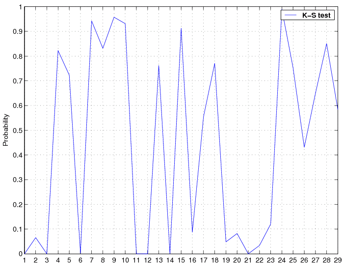
Figure 1: Quality of the EXPLORER data. The x-axis gives the number of the 11-hour block of data from the 13 day data run and the y-axis gives the corresponding probability values of the KS statistic.


Figure 2: Two-sided spectral density of the EXPLORER data.

3.3  Results

We have obtained 22 295 threshold crossings for the Northern hemisphere and 44 701 for the Southern hemisphere. We consider all candidates contained within a single cell of the parameter space defined in Section 2.2 as dependent and we choose as an independent candidate the candidate that has the highest signal-to-noise ratio within one cell. Consequently we have obtained 11 703 independent candidates for the Northern hemisphere and 18 702 for the Southern hemisphere. In Figures 3 and 4 we have plotted the histograms of the values of the statistics F for the independent candidates and we have compared it with the theoretical distribution for F when no signal is present in the data. A good agreement with the theoretical distribution is another indication of Gaussianity of the data. It also reveals that there are no obvious populations of the continuous gravitational-wave sources at the level of sensitivity of our search. In the search no event has crossed our 99% confidence threshold of 8.3. The strongest signal obtained by the coarse search had the signal-to-noise ratio of 7.9 and the fine search increased that value to 8.2.


Figure 3: Histogram of candidates: Northern hemisphere. On the x-axis the values of the statistic F are given.
The solid line corresponds to the theoretical c2 distribution with 4 degrees of freedom.


Figure 4: Histogram of candidates: Southern hemisphere. On the x-axis the values of the statistic F are given.
The solid line corresponds to the theoretical c2 distribution with 4 degrees of freedom.

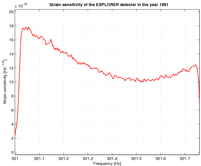
As we do not have a detection of a gravitational-wave signal we can make a statement about the upper bound for the gravitational-wave amplitude. To do this we take our strongest candidate of signal-to-noise ratio do and we suppose that it resulted from a gravitational-wave signal. Then, using formula (25), we calculate the signal-to-noise dul of the gravitational-wave signal so that there is 1% probability that it crosses the threshold Fo corresponding to do, where Fo = 2 + (1/2)d2o. The dul is the desired 99% confidence upper bound. For do = 8.2, which corresponds to the signal-to-noise ratio of our strongest candidate, we find that dul = 5.9. For the EXPLORER detector this corresponds to the dimensionless amplitude of the gravitational-wave signal equal to 2×10-23. Thus we have the following conclusion:

In the frequency band from 921.00 Hz to 921.76 Hz and for signals coming from any sky direction the dimensionless amplitude of the gravitational-wave signal from a continuous source is less than 2×10-23 with 99% confidence.
Our analysis has been done using two days of data. We note that the upper bound will decrease as length of the data analyzed increases; dul is proportional to the inverse of the square root of the observation time To.

Acknowledgments

The work of P. Jaranowski, A. Królak, K. M. Borkowski, and M. Pietka was supported in part by the KBN (Polish State Committee for Scientific Research) Grant No. 2P03B 094 17. The part of A. Królak research described in this paper was performed while he held an NRC-NASA Resident Research Associateship at the Jet Propulsion Laboratory, California Institute of Technology, under contract with the National Aeronautics and Space Administration. We would also like to thank Interdisciplinary Center for Mathematical and Computational Modeling of Warsaw University for computing time.

References

[1] Astone P et al. 1993 Phys. Rev. D 47 362
[2] Astone P et al. 2002 Phys. Rev. D 65 022001
[3] Jaranowski P, Królak A and Schutz B F 1998 Phys. Rev. D 58 063001
[4] Jaranowski P and Królak A 1999 Phys. Rev. D 59 063003
[5] Jaranowski P and Królak A 2000 Phys. Rev. D 61 062001
[6] Astone P, Borkowski K M, Jaranowski P and Królak A 2002 Phys. Rev. D 65 042003
[7] Lagarias J C, Reeds J A, Wright M H and Wright P E 1998 SIAM J. Optimization 9 112


Footnotes:

* On leave of absence from Institute of Mathematics Polish Academy of Sciences, Warsaw, Poland.
& krolak@jpl.nasa.gov
1 The EXPLORER detector is operated by the ROG collaboration located in Italian Istituto Nazionale di Fisica Nucleare (INFN); see www.roma1.infn.it/rog/explorer/explorer.html.


File translated from TEX by TTH, version 3.74 on 12 Jun 2006.